Example: MRI Application

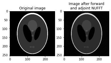
In this example we take an image of the Shepp-Logan phantom and we evaluate the forward NUFFT on a set of points defining a radial k-space trajectory. Then, we use the the adjoint NUFFT to recover the image from the radial k-space data.

Prepare data

Let’s begin by creating an example image. We will use a Shepp-Logan phantom, generated using TensorFlow MRI.

import tensorflow as tf
import tensorflow_mri as tfmri

grid_shape = [256, 256]
image = tfmri.image.phantom(shape=grid_shape, dtype=tf.complex64)

print("image: \n - shape: {}\n - dtype: {}".format(image.shape, image.dtype))

image: 
 - shape: (256, 256)
 - dtype: <dtype: 'complex64'>

Let us also create a k-space trajectory. In this example we will create a radial trajectory, also using TensorFlow MRI.

points = tfmri.sampling.radial_trajectory(base_resolution=256, views=233)
points = tf.reshape(points, [-1, 2])

print("points: \n - shape: {}\n - dtype: {}\n - range: [{}, {}]".format(
    points.shape, points.dtype,
    tf.math.reduce_min(points), tf.math.reduce_max(points)))

points: 
 - shape: (119296, 2)
 - dtype: <dtype: 'float32'>
 - range: [-3.1415927410125732, 3.141521453857422]

The trajectory should have shape [..., M, N], where M is the number of points and N is the number of dimensions. Any additional dimensions ... will be treated as batch dimensions.

Batch dimensions for image and traj, if any, will be broadcasted.

Spatial frequencies should be provided in radians/voxel, ie, in the range [-pi, pi].

Finally, we’ll also need density compensation weights for our set of nonuniform points. These are necessary in the adjoint transform, to compensate for the fact that the sampling density in a radial trajectory is not uniform. Here we use tensorflow-mri to calculate these weights.

weights = tfmri.sampling.radial_density(base_resolution=256, views=233)
weights = tf.reshape(weights, [-1])

print("weights: \n - shape: {}\n - dtype: {}".format(weights.shape, weights.dtype))

weights: 
 - shape: (119296,)
 - dtype: <dtype: 'float32'>

Forward transform (image to k-space)

Next, let’s calculate the k-space coefficients for the given image and trajectory points (image to k-space transform).

import tensorflow_nufft as tfft

kspace = tfft.nufft(image, points,
                    transform_type='type_2',
                    fft_direction='forward')

print("kspace: \n - shape: {}\n - dtype: {}".format(kspace.shape, kspace.dtype))

kspace: 
 - shape: (119296,)
 - dtype: <dtype: 'complex64'>

We are using a type-2 transform (uniform to nonuniform) and a forward FFT (image domain to frequency domain). These are the default values for transform_type and fft_direction, so providing them was not necessary in this case.

Adjoint transform (k-space to image)

We will now perform the adjoint transform to recover the image given the k-space data. In this case, we will use a type-1 transform (nonuniform to uniform) and a backward FFT (frequency domain to image domain). Also note that, prior to evaluating the NUFFT, we will compensate for the nonuniform sampling density by simply dividing the k-space samples by the density weights. Finally, for type-1 transforms we need to specify an additional grid_shape argument, which should be the size of the image. If there are any batch dimensions, grid_shape should not include them.

# Apply density compensation.
comp_kspace = kspace / tf.cast(weights, tf.complex64)

recon = tfft.nufft(comp_kspace, points,
                   grid_shape=grid_shape,
                   transform_type='type_1',
                   fft_direction='backward')

print("recon: \n - shape: {}\n - dtype: {}".format(recon.shape, recon.dtype))

recon: 
 - shape: (256, 256)
 - dtype: <dtype: 'complex64'>

Finally, let’s visualize the images.

import matplotlib.pyplot as plt

fig, ax = plt.subplots(1, 2)
ax[0].imshow(tf.abs(image), cmap='gray')
ax[0].set_title("Original image")
ax[1].imshow(tf.abs(recon), cmap='gray')
ax[1].set_title("Image after forward\nand adjoint NUFFT")

Text(0.5, 1.0, 'Image after forward\nand adjoint NUFFT')